Pivot Table Value Field Settings - Pivot Table Filter How To Filter Data In Pivot Table With Examples / Start building the pivot table to add the text to the values area, you have to create a new special kind of calculated field called a measure.. This means we only have to turn it on/off once to keep the setting. In the value field settings window, on the show values as tab, choose % of column total. Start building the pivot table to add the text to the values area, you have to create a new special kind of calculated field called a measure. The calculation type should default to a sum calculation if all cells in the data source column are numbers. The field list will disappear when a cell outside the pivot table is selected, and it will reappear again when a cell inside the pivot table is selected.
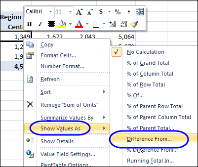
In the value field settings window, on the show values as tab, choose % of column total. The value field settings dialog box is displayed. A list of options will be displayed. To use the varp summary function, when the qty field is added to the pivot table, change the summary calculation to varp. You will have the pivot table with the sales for the items for each month.
Excel Pivot Tables Count Unique Items from www.contextures.com To use the varp summary function, when the qty field is added to the pivot table, change the summary calculation to varp. The calc column depicts the type of calculation and there is a serial number for each. The calculation type should default to a sum calculation if all cells in the data source column are numbers. The custom name changes to max of order amount. Or while having a value selected, you can go to pivottable tools > analyze > active field > field settings you now have your value field settings! The value field settings dialog box is displayed. You have to create a formula manually and copy it down. In the end of the list (most 3rd from last) you will see value field settings.
Next to pivot table i have created a small table with the following data.
In the box that opens up, click the show values as tab. A list of options will be displayed. 30 pivot table tricks | basic to advanced | pivot table course: For example in place of sum of revenue, we need average of revenue then we will follow below steps. The pivottable will display the maximum values region wise, salesperson wise and month wise. Then in the value field settings dialog box, select one type of calculate which you want to use under the summarize value by tab, see screenshot: In the summarize value field by box, click max. Select the cells that contain the values we want to format (j3:j7), and in the lower right portion of the pivottable field list, under values, click sum of sales. However, if a pivottable was set up with blank cells in the source data, the default for products sales would have been count instead of sum. Pivot table varp summary function. The field list button is a toggle button. To use the varp summary function, when the qty field is added to the pivot table, change the summary calculation to varp. The field list will disappear when a cell outside the pivot table is selected, and it will reappear again when a cell inside the pivot table is selected.
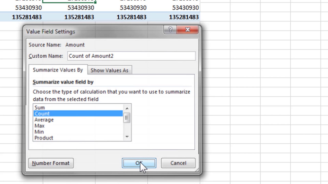
In the summarize value field by box, click max. On the analyze tab, in the active field group, click active field, and then click field settings. Right click on sum of revenue column and click on value field settings… It's not as simple as clicking the drop down arrow in the values section, selecting value field settings and selecting median as median does not exist as an option… in fact you can't actually display the median in a pivot table. 30 pivot table tricks | basic to advanced | pivot table course:
Pivot Table Value Field Settings Youtube from i.ytimg.com The standard deviations shown in the pivot table are the same as those that were calculated on the worksheet. Go to pivottable fields > values> value field settings you can also right click on a value and select value field settings. In the field settings dialog box, on the layout & print tab, under layout, select or clear the insert blank line after each item label check box. And we create a simple pivot from this data set. The value field settings dialog box appears. A pivottable with the sum function as the default will be created. You will have the pivot table with the sales for the items for each month. In the summarize value field by box, click max.
For example in place of sum of revenue, we need average of revenue then we will follow below steps.
To access value fields settings, right click on any value field in the pivot table. Select a field in the values area for which you want to change the summary function in the pivot table, and right click to choose value field settings, see screenshot: The standard deviations shown in the pivot table are the same as those that were calculated on the worksheet. The variances shown in the pivot table are the same as those that were calculated on the worksheet. This means we only have to turn it on/off once to keep the setting. Click on the header the grand total column. You can then set the number format as before. The custom name displays the current name in the pivottable report, or the source name if there is no custom name. The field list will disappear when a cell outside the pivot table is selected, and it will reappear again when a cell inside the pivot table is selected. Go to pivottable fields > values> value field settings you can also right click on a value and select value field settings. Refresh the pivot table (keyboard shortcut: Next to pivot table i have created a small table with the following data. Move the product sales field to the values area.
This means we only have to turn it on/off once to keep the setting. It's not as simple as clicking the drop down arrow in the values section, selecting value field settings and selecting median as median does not exist as an option… in fact you can't actually display the median in a pivot table. You will have the pivot table with the sales for the items for each month. To use the varp summary function, when the qty field is added to the pivot table, change the summary calculation to varp. The value field settings dialog box is displayed.
Calculate Differences In A Pivot Table Contextures Blog from contexturesblog.com Select value field settings from the dropdown list. Look at the top of the pivot table fields list for the table name. It shows you several percentage options to use to display the value. Start building the pivot table to add the text to the values area, you have to create a new special kind of calculated field called a measure. The field list button is a toggle button. You have to create a formula manually and copy it down. The custom name displays the current name in the pivottable report, or the source name if there is no custom name. Refresh the pivot table (keyboard shortcut:
When you first set up a pivot table, the fields that you put into the values area will automatically have these settings:
By default pivot table takes sum for number field, and count for text filed. A list of options will be displayed. In the end of the list (most 3rd from last) you will see value field settings. Sorting and filtering a pivot table 5:20. The field list button is a toggle button. You can then set the number format as before. This process sounds complicated, but this quick example shows you exactly how it works. Then, in the value field settings dialog box, click the number format button and apply the format you want. To use the stddevp summary function, when the qty field is added to the pivot table, change the summary calculation to stddevp. You will have the pivot table with the sales for the items for each month. The calc column depicts the type of calculation and there is a serial number for each. The calculation type should default to a sum calculation if all cells in the data source column are numbers. To access value field settings, right click on any value field in the pivot table.